Introduction to INT8 quantization in JAX

Introduction

In this blog post, we will provide an intuitive introduction to a technique called quantization. The topic has always seemed a bit mysterious to me because, in most modern ML packages, you only need to make a specification in the training config, and the rest is done for you without really understanding what is going on. In the following, we will try to shed some light on quantization by explicitly writing out an example from scratch.

Our example

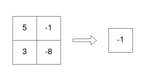
To focus on the topic at hand we will take a very simple example: Consider a quadratic Matrix A. We will simply sum up all the elements in the matrix and see how much speedup we can archieve (or not) by quantizing the input. For people that like visualizations our program will do the following

Float 32 (no quantization)

In Jax we can initialize a matrix with entries all drawn from a normal distribution as follows:

import jax
from timing_util import simple_timeit
import numpy

n_rows, n_cols = 32_768, 32_768

A = numpy.random.randn(n_rows * n_cols)

A_f32 = jax.numpy.asarray(A, dtype=jax.numpy.float32).reshape( (n_rows, n_cols) )

As we see the dtype here is float32, that means we have 4 bytes to express each entry in the matrix. Summing the entries is as easy as

@jax.jit
def sum_f32(arr):
    return jax.numpy.sum(arr)

We can use the timeit function which you can find here to measure how long it takes. To compare the numerical accuracies we should also save the output in a variable. We can do this as follows:

t_float_32 = simple_timeit(sum_f32, A_f32, tries=30, task="sum_float_32")
out_float_32 = sum_f32(A_f32)

Bfloat 16 (simple quantization)

A first step to quantize would be very simple: Just use bfloat16 which uses 2 bytes to represent every entry in the matrix. For a simple introduction on how bfloat16 differs from float32 see this link. Transfering our code to use bfloat16 is as simple as this:

A_b16 = jax.numpy.asarray(A, dtype=jax.numpy.bfloat16).reshape( (n_rows, n_cols) )

@jax.jit
def sum_bf16(arr):
    return jax.numpy.sum(arr)

t_bfloat_16 = simple_timeit(sum_bf16, A_b16, tries=30, task="sum_bfloat_16")
out_bfloat_16 = sum_bf16(A_b16)

For the example above, this already gives a good speedup on a TPU-v4-8. If we calculate the relative difference in time and the sum, we obtain:

1-t_bfloat_16/t_float_32 =0.34623850537246814
1-out_bfloat_16/out_float_32 =Array(0.00167018, dtype=float32)

We can see that we get a speedup of 34% while only sacrificing a little bit of accuracy and with minimal adjustments in code.

Int 8

It turns out that modern TPUs are very efficent in carrying out calculation in int8. Now we need to ask ourselves how we can convert the floating point numbers which are the entries to our matrix to integers ranging from -127 to 127. It turns out there is a simple algorithm to archieve that goal. Let’s consider a matrix and call the scale of the matrix the maximum of the absolute values of the matrix entries. We can visualize it like this:

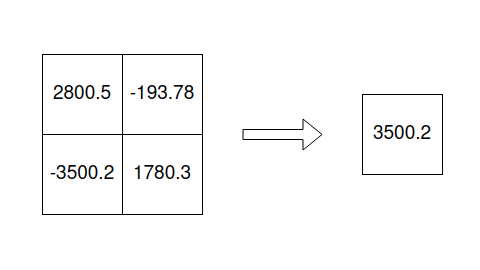
Obviously we can use the scale to normalize our matrix, i.e. we squash all entries to be between -1 and 1. We then multiply by 127 to obtain floating points between -127 and 127. This will be casted to int8and we are ready to make our in int8. See below for the intermediate output:

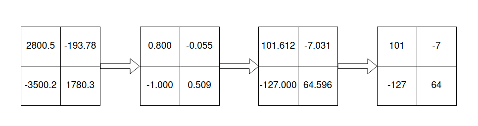
Let us call our original matrix M and our int8 matrix N. From the above we see that approximately N is equal to M times the scaling factor of 127/max(abs(M)) which means that after summing up the entries of N we need to multiply by max(abs(M))/127 to get an approximation of sum(M). Obviously this step will cast our output implicitly back to float32. To give the full code in jax:

scale = jax.numpy.max( jax.numpy.abs(A_f32) )
A_i8 = jax.numpy.asarray( A_f32 / scale * 127, dtype=jax.numpy.int8)

@jax.jit
def sum_int8(scaled_arr, scale):
    out = jax.numpy.sum(scaled_arr)
    return out * scale / 127

t_int_8 = simple_timeit(sum_int8, A_i8, scale, tries=30, task="sum_int_8")
out_int_8 = sum_int8(A_i8, scale)

The result is impressive:

1-t_int_8/t_bfloat_16 =0.5729217991131133
1-out_int_8/out_float_32 =Array(0.02700579, dtype=float32)

That means we get a huge speedup of 57% compared to bfloat16 while still being relatively accurate.

Further considerations

One could ask, how the above numbers change for different values of the n_rows=n_cols=MATRIX_SIZE. Find the result below:

MATRIX_SIZE =8192
1-t_bfloat_16/t_float_32 =0.4849284741144412
1-t_int_8/t_bfloat_16 =-0.019507356587865843
MATRIX_SIZE =16384
1-t_bfloat_16/t_float_32 =0.32089008463651136
1-t_int_8/t_bfloat_16 =0.4819247276328822
MATRIX_SIZE =32768
1-t_bfloat_16/t_float_32 =0.3467612778641981
1-t_int_8/t_bfloat_16 =0.5689701690382064

We see that the speedup is largely dependent on the number of entries. That means in practice we need to be careful (at least on a TPU-v4-8) how to quantize.

Conclusion

In this blogpost we saw how INT8 quantization can give us huge speedups when running matrix calculations on a TPU. For further background you might find this blogpost interesting. The experiments shown here were supported by the TRC research program.