Multi chip performance in JAX

The larger the models we use get the more it becomes necessary to be able to perform training of machine learning models over multiple chips. In this blog post we will explain how to efficiently use Google’s TPU. TPUs are especially convenient as they are designed especially for machine learning and easily deployable on Google Cloud. For an introduction on how to deploy your own TPU with Google Cloud, see this excellent documentation.

In this tutorial we will take a simple layerwise matrix multiplication of activations with weights as our running example. The workload may be visualized like this:

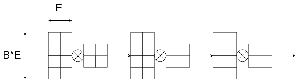
In the above diagram the activations have shape B*E x E and the weights have shape E x E. The question is now how we can distribute this workload in an efficent way onto the different TPU chips.

For the activations it’s pretty obvious how we can distribute them onto different chips: Just put each batch onto one chip and then run the calculation for each batch independently, that is we multiply each batch with the weights matrix. This can be visualized as follows: 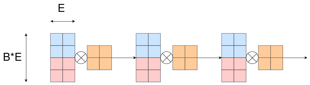The different colors should visualize the fact that the activations are distributed batchwise over the different chips and the weights are copied onto all chips. In JAX we can accomplish distribution onto different chips as follows:

import jax
from timing_util import simple_timeit

### Parameters
MATRIX_SIZE = 16_384

A = jax.numpy.ones((MATRIX_SIZE, MATRIX_SIZE), dtype=jax.numpy.bfloat16)

### Create our shard
mesh = jax.sharding.Mesh(jax.devices(), ("axis"))
p = jax.sharding.PartitionSpec(None, "axis")
sharding = jax.sharding.NamedSharding(mesh, p)

### shard the array
A_sharded = jax.device_put(A, sharding)

### Visualize the sharding
print(f"{p=}")
print(f"{A_sharded.shape=}, {A_sharded.addressable_shards[0].data.shape=}")
jax.debug.visualize_array_sharding(A_sharded)

Depending on how we define the partitioning we will get the following:

p=PartitionSpec(None, 'axis')
A_sharded.shape=(16384, 16384), A_sharded.addressable_shards[0].data.shape=(16384, 4096)
┌───────┬───────┬───────┬───────┐
│       │       │       │       │
│       │       │       │       │
│       │       │       │       │
│       │       │       │       │
│ TPU 0 │ TPU 1 │ TPU 2 │ TPU 3 │
│       │       │       │       │
│       │       │       │       │
│       │       │       │       │
│       │       │       │       │
└───────┴───────┴───────┴───────┘

p=PartitionSpec('axis', None)
A_sharded.shape=(16384, 16384), A_sharded.addressable_shards[0].data.shape=(4096, 16384)
┌───────────────────────┐
│         TPU 0         │
├───────────────────────┤
│         TPU 1         │
├───────────────────────┤
│         TPU 2         │
├───────────────────────┤
│         TPU 3         │
└───────────────────────┘

p=PartitionSpec(None,)
A_sharded.shape=(16384, 16384), A_sharded.addressable_shards[0].data.shape=(16384, 16384)
┌───────────────────────┐
│                       │
│                       │
│                       │
│                       │
│      TPU 0,1,2,3      │
│                       │
│                       │
│                       │
│                       │
└───────────────────────┘

We see that we want to use the partition p=PartitionSpec('axis', None) for the activations and p=PartitionSpec(None,) for the weights.

So far so good but this still doesn’t leverage the full power of having multiple chips. What if the weight matrices are very large- So large that we can’t distribute all of them onto each chip?

It turns out we can do the following: 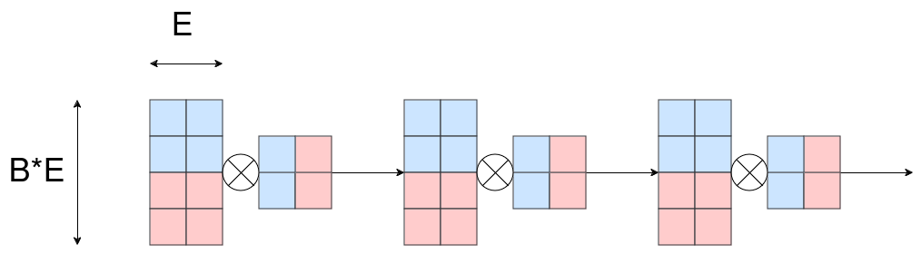What we see is that initially we distribute the weights also over all available chips. But for the calculation we need the weight for the current layer to be on all chips. How can this be archieved? It turns out the algorithm is quiete simple: Let L_i, A_i, W_i be i-th layer, activation and weight. While calculating L_{i+1}, i.e. multiplying A_i with W_i we have W_i ungathered (i.e. distributed over all chips). At the same time we ungather W_{i+1}. When done with L_i we can distribute W_i back onto all chips. If this process is faster than the matrix multiplication we only need to keep 2 weights unsharded instead of N_layer weights while not decreasing performance! Let’s see how we can implement that in JAX:

import jax
from timing_util import simple_timeit

### Parameters
BATCH_PER_CHIP = 4096
MATRIX_SIZE = 16_384
N_LAYERS = 4

### Activations and weights
ACTIVATION = jax.numpy.ones((BATCH_PER_CHIP*jax.device_count(), MATRIX_SIZE), dtype=jax.numpy.bfloat16)
WEIGHTS = [jax.numpy.ones((MATRIX_SIZE, MATRIX_SIZE), dtype=jax.numpy.bfloat16) for _ in range(N_LAYERS)]

### Shardings 
mesh = jax.sharding.Mesh(jax.devices(), ("axis"))
### Distribute data along the rows
p_a = jax.sharding.PartitionSpec("axis", None)
### Distribute data along the columns
p_w = jax.sharding.PartitionSpec(None, "axis")

sharding_a = jax.sharding.NamedSharding(mesh, p_a)
sharding_w = jax.sharding.NamedSharding(mesh, p_w)

### Shard the activations
ACTIVATION = jax.device_put(ACTIVATION, sharding_a)
WEIGHTS = [jax.device_put(w, sharding_w) for w in WEIGHTS]

### Let jax determine how to perform the forward pass efficiently
@jax.jit
def matmul(ACTIVATION, WEIGHTS):
    for w in WEIGHTS:
        ACTIVATION = ACTIVATION @ w
    return ACTIVATION

### Time the forward pass
average_time = simple_timeit(matmul, ACTIVATION, WEIGHTS, task="matmul")

print(f"Average time for forward pass: {average_time:.2f} ms")

For the above setting we archieved an average time of 39.82 ms on Googles TPU-v4-8 (that is a TPU with 8/2=4 chips).

Let’s look at the trace viewer to get more insight about how jax compiled the matmul function: We see that JAX does exactly what we described above! Only the first all gather is performed for a “long” time. Afterwards the gathering process gets fused with the matrix multiplication which gives a huge speedup if we compare it to the naive approach that we would just apply all gathering after each matrix multiplication and at the same time it gives us the benefit that we can safe lots of memory by sharding most of the weights over all chips. Keep in mind that this compilation won’t be done by default on a TPU of the fourth generation. To get this speedup we need to execute export LIBTPU_INIT_ARGS="--xla_enable_async_all_gather=true TPU_MEGACORE=MEGACORE_DENSE" in our terminal to initialize the TPU correctly. If you won’t do that the all gathering won’t be fused with the matmul and as a result it will take around 53.31 ms.

I hope this post was insightful and you liked it. Large parts of it are based on the insights from this fantastic online course delivered by Rafi Witten. The code for the timeit function can be found in this repo aswell. The experiments were supported by Googles TRC program